Optimal RANSAC

Background

Optimal RANSAC is a repeatable variant of the RANSAC algorithm introduced by Hast et al. (2013). Standard RANSAC is inherently non-deterministic: because it selects random minimal samples, two runs on the same data can find different inlier sets, which is problematic when the algorithm is embedded in a larger pipeline that must be reproducible. Optimal RANSAC addresses this by augmenting the standard hypothesis-and-verify loop with three iterative refinement steps that steer the search toward the global optimal inlier set, making repeated convergence to the same result much more likely than in the standard RANSAC algorithm.

The algorithm

Optimal RANSAC shares its outer structure with standard RANSAC but, crucially, replaces the single scoring step with three tightly coupled sub-procedures whenever a candidate hypothesis yields more than a small number of tentative inliers.

1. Resample (Algorithm 2)

A random subset of up to a quarter of the current tentative-inlier set is drawn and a new model is fitted to that subset. The new model is then scored against the full dataset using a (optionally wider) search tolerance $t_{\mathrm{search}}$. If this produces a larger inlier set the resampling loop restarts from the expanded set; otherwise it tries up to 8 different subsets before returning. This is directly inspired by the Local-Optimisation step of LO-RANSAC (Chum et al., 2003; Chum et al., 2004) but is triggered more aggressively: whenever a promising hypothesis is found rather than only after a global best is updated.

2. Rescore (Algorithm 3)

Starting from the inlier set produced by resampling, the model is iteratively re-estimated from all current inliers and scored against all data until the inlier set stops changing or after at most 20 iterations. Using all inliers for fitting (rather than only the minimal sample $s$) exploits the fact that many problems admit a least-squares fit from more than $s$ points, producing a model that is better aligned to the true structure.

3. Pruneset (Algorithm 4) — optional

When a wider search tolerance $t_{\mathrm{search}} > t$ is used alongside a distfn input that returns per-point residuals, a final pruning pass removes any inlier whose residual exceeds the tight tolerance $t$. The most extreme inlier is removed one at a time and the model is re-estimated after each removal, so that the final model is always consistent with the retained inliers.

Stopping criterion

Instead of the adaptive $N$ iterations formula used by standard RANSAC, Optimal RANSAC terminates when the same inlier-set size is re-discovered a specified number of times in succession (min_consensus, default 2). The refinement steps make it very unlikely to find the same size by chance unless it corresponds to the true optimal set, so this simple criterion works surprisingly well in practice. This is the main convergence criterion for Optimal RANSAC; increasing min_consensus is recommended if the default value does not reliably reproduce the same inlier set and is typically most necessary when the tentative number of inliers per trial is low (this information is shown if you set the keyword argument verbose = true).

When to use Optimal RANSAC

The runtime of Optimal RANSAC is generally longer than standard RANSAC as it typically makes more calls to distfn and fittingfn per data trial. Additionally, fittingfn must support overconstrained problems which require more computation to solve than minimally-constrained problems as expected in standard RANSAC, so calls to fittingfn may be much more expensive if your dataset is large. For small problems (e.g., simple line fitting) this additional cost is often negligible and Optimal RANSAC may be preferred for its robustness and repeatibility. Optimal RANSAC may be preferrable to standard RANSAC when:

• repeatability is important regardless of RNG state (standard RANSAC is repeatible given the same seeded RNG, but generally not otherwise, while Optimal RANSAC is designed to be repeatible regardless of RNG state),
• fittingfn supports overconstrained fits with more than s points (required for the rescoring step),
• the inlier fraction is very low (well below 5%), making RANSAC's standard adaptive stopping criterion unreliable, or
• a high-precision final inlier set is needed (using the two-tolerance mode with t_search > t).

API

optimalransac(x, fittingfn, distfn, s, t;
              rng = Random.default_rng(),
              t_search = t,
              degenfn = _ -> false,
              verbose = false,
              max_data_trials = 100,
              max_trials = 1000,
              min_inliers = 5,
              min_consensus = 2)

Example: fitting a line in the presence of outliers

The following example generates 100 inlier points near the line $y = 2x + 3$, adds 100 outliers scattered over a wider region, and uses Optimal RANSAC to recover the true parameters.

using ConsensusFitting
using Random
using CairoMakie

Random.seed!(42)

# ── Generate synthetic data ────────────────────────────────────────────────
a_true, b_true = 2.0, 3.0
n_inliers  = 100
n_outliers = 100

x_in = collect(range(-10.0, 10.0; length=n_inliers))
y_in = a_true .* x_in .+ b_true .+ randn(n_inliers)

x_out = -10.0 .+ 20.0 .* rand(n_outliers)
y_out = -25.0 .+ 50.0 .* rand(n_outliers)

# Pack into a 2 × N matrix (each column is one data point [x; y])
data = [vcat(x_in, x_out)'; vcat(y_in, y_out)']

# ── Define the fitting and distance functions ──────────────────────────────

# Fit a line y = a*x + b
function fit_line(pts)
    n = size(pts, 2)
    n < 2 && return []
    if n == 2
        # If minimally constrained,
        x1, y1 = pts[1, 1], pts[2, 1]
        x2, y2 = pts[1, 2], pts[2, 2]
        isapprox(x1, x2; atol=1e-10) && return []
        a = (y2 - y1) / (x2 - x1)
        b = y1 - a * x1
        return [a, b]
    else
        # If overconstrained, least-squares fit
        A = hcat(pts[1, :], ones(n))
        b = pts[2, :]
        coef = A \ b
        return [coef[1], coef[2]]
    end
end

# Classify points using their vertical (y-direction) residual.
function line_dist(M, x, t)
    a, b    = M[1], M[2]
    resid   = abs.(x[2, :] .- (a .* x[1, :] .+ b))
    inliers = findall(resid .< t)
    return (model=M, inliers=inliers, residuals=resid)
end

# Run Optimal RANSAC with pruning
M, inliers = optimalransac(data, fit_line, line_dist, 2, 2.0; t_search=4.0, min_consensus=10)

println("Recovered slope:     ", round(M[1]; digits=4), "  (true: $a_true)")
println("Recovered intercept: ", round(M[2]; digits=4), "  (true: $b_true)")
println("Inliers identified:  ", length(inliers), " / $(size(data, 2))")

Recovered slope:     1.9718  (true: 2.0)
Recovered intercept: 2.8728  (true: 3.0)
Inliers identified:  108 / 200

Visualising the result

outlier_mask = trues(size(data, 2))
outlier_mask[inliers] .= false

fig = Figure(size=(500, 500))
ax  = Axis(fig[1, 1];
           xlabel="x", ylabel="y",
           title="Optimal RANSAC line fitting")

# All data points
scatter!(ax, data[1, outlier_mask], data[2, outlier_mask];
         color=(:tomato, 0.7), markersize=8, label="Outliers")
scatter!(ax, data[1, inliers], data[2, inliers];
         color=(:steelblue, 0.8), markersize=8, label="Inliers")

# True and recovered lines
x_plot = range(-10.0, 10.0; length=200)
lines!(ax, x_plot, M[1] .* x_plot .+ M[2];
       color=:orange, linewidth=2.5, label="Optimal RANSAC fit")
lines!(ax, x_plot, a_true .* x_plot .+ b_true;
       color=:black, linewidth=2, linestyle=:dash, label="True line")

axislegend(ax; position=:lt)
fig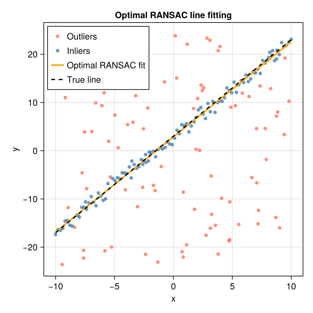

Generally a "finalizer" step (doing a final fit to the set of all inliers) is redundant with Optimal RANSAC, as this is already what is returned. Here we will just redo the fit with the inliers to additionally estimate parameter uncertainties. You will see that the best-fit values found μ are the same as what was output in M above.

using LinearAlgebra: dot

"""
    fit_line_overconstrained(data)

Fit a line y = a + b*x to data given as a 2×N matrix:
    data[1, :] = x
    data[2, :] = y

# Returns
  - `θ` :[a, b] (slope, intercept)
  - `Σθ`: covariance matrix of θ (2×2)
  - `σ²`: estimated residual variance
"""
function fit_line_overconstrained(data)
    @assert size(data, 1) == 2 "Input must be a 2×N matrix"
    x = view(data, 1, :)
    y = view(data, 2, :)
    N = length(x)
    @assert N ≥ 2 "Need at least two points"
    # Least-squares solution
    A = hcat(x, ones(N)) # Design matrix: [x 1]
    θ = A \ y   # equivalent to (A'A)^(-1)A'y but more stable
    r = y - A * θ # Residuals
    # Degrees of freedom: N - number of parameters (2)
    dof = N - 2
    @assert dof > 0 "Need more than 2 points for covariance estimate"
    # Residual variance estimate
    σ² = dot(r, r) / dof
    # Covariance matrix: σ² * (A'A)^(-1)
    Σθ = σ² * inv(A' * A)
    return θ, Σθ, σ²
end

μ, Σθ, σ² = fit_line_overconstrained(data[:, inliers])
println("Recovered slope:     ", round(μ[1]; digits=4), " ± ", round(sqrt(Σθ[1,1]); digits=4), "  (true: $a_true)")
println("Recovered intercept:     ", round(μ[2]; digits=4), " ± ", round(sqrt(Σθ[2,2]); digits=4), "  (true: $b_true)")
println("M == μ:     ", M == μ)

Recovered slope:     1.9718 ± 0.0145  (true: 2.0)
Recovered intercept:     2.8728 ± 0.0849  (true: 3.0)
M == μ:     true

References

This page cites the following references: