IUSAC

Background

IUSAC (Iterative Update Sample Consensus) is a repeatable variant of the RANSAC algorithm introduced by Kim et al. (2024). Like Optimal RANSAC, it addresses the fundamental non-determinism of standard RANSAC by augmenting the hypothesis-and-verify loop with an iterative update step that steers each candidate toward the globally optimal inlier set.

The key insight of IUSAC is that once an initial hypothesis is "close enough" to the true model, iteratively re-estimating the model from the full current inlier set (rather than from only the minimal sample) and rescoring against all data will cause the consensus set to grow monotonically until convergence. This is backed by a formal convergence analysis in Kim et al. (2024): when the objective function is locally quadratic around the true solution (which holds for least-squares problems under mild regularity conditions), the iterative update is equivalent to one step of Newton's method and is guaranteed to decrease the residual.

The algorithm

Given a dataset $X$ of $N$ points, a minimum sample size $s$, an inlier distance threshold $\tau_e$, a stopping threshold $\hat{\eta}$, and a convergence tolerance $\varepsilon$, our implementation of IUSAC proceeds as follows:

1. Initialization – outer loop — for each iteration of the outer loop, draw a random minimal sample of $s$ points and fit a candidate model $p_0$. Score it against all data to obtain the initial consensus set $C_0 = \operatorname{inlier}(X, p_0, \tau_e)$. Strategies for the initialization can vary; here we adopt a standard RANSAC approach for the initialization (see RANSAC), generating the initial hypotheses in an outer RANSAC loop with its own convergence criterion (p). The outer RANSAC loop generates increasingly likely hypotheses for input to the inner IUSAC loop, which is necessary as the convergence of IUSAC depends on an initial hypothesis "close" to the true model.

2. Iterative update – inner loop — starting from $C_0$, repeat:

   • (a) Re-estimate the model from all current inliers: $p_k = g(C_{k-1})$.
   • (b) Rescore against all data: $C_k = \operatorname{inlier}(X, p_k, \tau_e)$.
   • (c) Convergence check:
     • If $|C_k| < |C_{k-1}|$: set $C^* = C_{k-1}$ and stop. The consensus set has shrunk, so the previous set was better.
     • If $|C_k| < (1 + \varepsilon)|C_{k-1}|$: set $C^* = C_k$ and stop. Growth has stagnated (relative increase below $\varepsilon = 0.001$); this generally only triggers when the number of inliers is high.
     • Otherwise: continue with $C_{k-1} \leftarrow C_k$.

3. Stopping criterion – inner loop — if $|C^*| \geq \hat{\eta} N$, re-estimate $p^* = g(C^*)$ and terminate inner loop. Otherwise, repeat steps 2–3 a number of times (keyword argument max_inner_iterations).

4. Stopping criterion – outer loop As our outer loop is a standard RANSAC, we use the standard RANSAC stopping criterion, where the number of outer iterations $N_{out}$ is updated adaptively as

   \[N = \frac{\log(1 - p)}{\log\!\left(1 - \left(\varepsilon_{\mathrm{in}}\right)^s\right)}\]

   where $\varepsilon_{\mathrm{in}}$ is the current best estimate of the inlier fraction and $s$ is the minimum sample size. The algorithm also supports an explicit early-stop threshold eta_b, which will terminate the outer loop when $\varepsilon_{\mathrm{in}} ≥ \varepsilon_b$.

Why it is repeatable

The iterative update reliably expands any "good enough" initial hypothesis to the global optimal inlier set, because re-estimating from all current inliers produces a model that is better aligned to the true structure than one fitted to only $s$ points. As long as the RANSAC-style random sampling produces at least one outer iteration whose initial consensus set overlaps sufficiently with the true inlier set, the iterative update will guide that iteration to the optimal solution. The probability of this happening increases with the number of outer trials, making IUSAC highly repeatable in practice.

When to use IUSAC

As IUSAC is essentially RANSAC with an additional inner iteration loop, the runtime is generally longer than standard RANSAC as it typically makes more calls to distfn and fittingfn per data trial. However, IUSAC may converge with fewer outer RANSAC iterations, so often it is not much more expensive than standard RANSAC. However, fittingfn must support overconstrained problems which require more computation to solve than minimally-constrained problems as expected in standard RANSAC, so calls to fittingfn may be more expensive if your dataset is large. For small problems (e.g., simple line fitting) this additional cost is often negligible and IUSAC may be preferred for its robustness and repeatibility. IUSAC may be preferrable to standard RANSAC when:

• repeatability across runs (with different random seeds) is important,
• the inlier fraction is moderate ($\sim 30\%$ or more),
• fittingfn supports overconstrained fits with more than s points (required for the iterative update step).

IUSAC is less suitable when:

• the model fitting step does not support over-determined inputs,
• the inlier fraction is extremely low ($\lesssim 5\%$), where the outer loop will rarely produce a good initialisation,
• multiple competing structures of similar quality are present.

API

iusac(x, fittingfn, distfn, s, t;
      rng = Random.default_rng(),
      degenfn = _ -> false,
      verbose = false,
      verbose_io = stdout,
      max_data_trials = 100,
      max_trials = 1000,
      p = 0.99,
      eta_b = 1.0,
      epsilon = 0.001,
      max_inner_iterations = 100)

Example: fitting a line in the presence of outliers

The following example generates 100 inlier points near the line $y = 2x + 3$, adds 100 outliers scattered over a wider region, and uses IUSAC to recover the true parameters.

using ConsensusFitting
using Random
using CairoMakie

Random.seed!(42)

# ── Generate synthetic data ────────────────────────────────────────────────
a_true, b_true = 2.0, 3.0
n_inliers  = 100
n_outliers = 100

x_in = collect(range(-10.0, 10.0; length=n_inliers))
y_in = a_true .* x_in .+ b_true .+ randn(n_inliers)

x_out = -10.0 .+ 20.0 .* rand(n_outliers)
y_out = -25.0 .+ 50.0 .* rand(n_outliers)

# Pack into a 2 × N matrix (each column is one data point [x; y])
data = [vcat(x_in, x_out)'; vcat(y_in, y_out)']

# ── Define the fitting and distance functions ──────────────────────────────

# Fit a line y = a*x + b through ≥ 2 points.
function fit_line(pts)
    n = size(pts, 2)
    n < 2 && return []
    if n == 2
        # Minimally constrained: two-point exact fit
        x1, y1 = pts[1, 1], pts[2, 1]
        x2, y2 = pts[1, 2], pts[2, 2]
        isapprox(x1, x2; atol=1e-10) && return []   # vertical line → degenerate
        a = (y2 - y1) / (x2 - x1)
        b = y1 - a * x1
        return [a, b]
    else
        # Over-constrained: least-squares fit (required for iterative update)
        A = hcat(pts[1, :], ones(n))
        b = pts[2, :]
        coef = A \ b
        return [coef[1], coef[2]]
    end
end

# Classify points using their vertical (y-direction) residual.
function line_dist(M, x, t)
    a, b    = M[1], M[2]
    resid   = abs.(x[2, :] .- (a .* x[1, :] .+ b))
    inliers = findall(resid .< t)
    return (model=M, inliers=inliers)
end

# ── Run IUSAC ──────────────────────────────────────────────────────────────
M, inliers = iusac(data, fit_line, line_dist, 2, 2.0)

println("Recovered slope:     ", round(M[1]; digits=4), "  (true: $a_true)")
println("Recovered intercept: ", round(M[2]; digits=4), "  (true: $b_true)")
println("Inliers identified:  ", length(inliers), " / $(size(data, 2))")

Recovered slope:     1.9685  (true: 2.0)
Recovered intercept: 2.8938  (true: 3.0)
Inliers identified:  109 / 200

Visualising the result

outlier_mask = trues(size(data, 2))
outlier_mask[inliers] .= false

fig = Figure(size=(500, 500))
ax  = Axis(fig[1, 1];
           xlabel="x", ylabel="y",
           title="IUSAC line fitting")

# All data points
scatter!(ax, data[1, outlier_mask], data[2, outlier_mask];
         color=(:tomato, 0.7), markersize=8, label="Outliers")
scatter!(ax, data[1, inliers], data[2, inliers];
         color=(:steelblue, 0.8), markersize=8, label="Inliers")

# True and recovered lines
x_plot = range(-10.0, 10.0; length=200)
lines!(ax, x_plot, M[1] .* x_plot .+ M[2];
       color=:orange, linewidth=2.5, label="IUSAC fit")
lines!(ax, x_plot, a_true .* x_plot .+ b_true;
       color=:black, linewidth=2, linestyle=:dash, label="True line")

axislegend(ax; position=:lt)
fig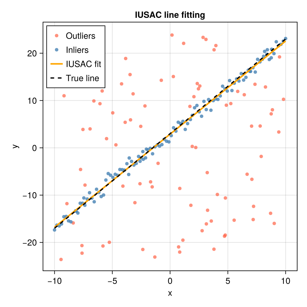

Because the iterative update re-estimates the model when the list of inliers is expanded, M already represents the fit to the identified inlier set and no separate "finalizer" step is needed. Here we will just redo the fit with the inliers to additionally estimate parameter uncertainties. You will see that the best-fit values found μ are the same as what was output in M above.

using LinearAlgebra: dot

"""
    fit_line_overconstrained(data)

Fit a line y = a + b*x to data given as a 2×N matrix:
    data[1, :] = x
    data[2, :] = y

# Returns
  - `θ` :[a, b] (slope, intercept)
  - `Σθ`: covariance matrix of θ (2×2)
  - `σ²`: estimated residual variance
"""
function fit_line_overconstrained(data)
    @assert size(data, 1) == 2 "Input must be a 2×N matrix"
    x = view(data, 1, :)
    y = view(data, 2, :)
    N = length(x)
    @assert N ≥ 2 "Need at least two points"
    A = hcat(x, ones(N))
    θ = A \ y
    r = y - A * θ
    dof = N - 2
    @assert dof > 0 "Need more than 2 points for covariance estimate"
    σ² = dot(r, r) / dof
    Σθ = σ² * inv(A' * A)
    return θ, Σθ, σ²
end

μ, Σθ, σ² = fit_line_overconstrained(data[:, inliers])
println("Recovered slope:     ", round(μ[1]; digits=4), " ± ", round(sqrt(Σθ[1,1]); digits=4), "  (true: $a_true)")
println("Recovered intercept: ", round(μ[2]; digits=4), " ± ", round(sqrt(Σθ[2,2]); digits=4), "  (true: $b_true)")
println("M == μ:     ", M == μ)

Recovered slope:     1.9685 ± 0.0148  (true: 2.0)
Recovered intercept: 2.8938 ± 0.0866  (true: 3.0)
M == μ:     true

References

This page cites the following references: