Morphological Operations
![]()

Morphological image processing is an area of computer vision which pursues to remove imperfections from binary and grayscale images.
ImageMorphology.jl holds a collection of non-linear operations related to the shape or morphology of features in an image.
In this demonstration, we'll cover the 8 most common morphological operations:
- Erosion
- Dilation
- Opening
- Closing
- Tophat
- Bothat
- Morphological Gradient
- Morphological Laplace
Let's import an image
using Images
using ImageMorphology, TestImages

img = Gray.(testimage("morphology_test_512"))
Erosion
Erode performs a min-filter over its nearest-neighbors. The default is 8-connectivity in 2d, 27-connectivity in 3d, etc. You can specify the list of dimensions that you want to include in the connectivity, e.g., region = [1,2] would exclude the third dimension from filtering.
Below example shows how erosion works on a binary image using 3x3 structuring element. The 3x3 size structuring element checks neighbours for every pixel in the original image to update that pixel's value with minimum of the neighbours in the resultant image .
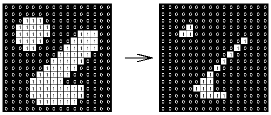
img_erode = @. Gray(img < 0.8); # keeps white objects white
img_erosion1 = erode(img_erode)
img_erosion2 = erode(erode(img_erode))
mosaicview(img_erode, img_erosion1, img_erosion2; nrow = 1)
Dilation
Dilate performs a max-filter over its nearest-neighbors. The default is 8-connectivity in 2d, 27-connectivity in 3d, etc. You can specify the list of dimensions that you want to include in the connectivity, e.g., region = [1,2] would exclude the third dimension from filtering.
Below example shows how dilation works on a binary image using 3x3 structuring element. The 3x3 size structuring element checks neighbours for every pixel in the original image to update that pixel's value with maximum of the neighbours in the resultant image .
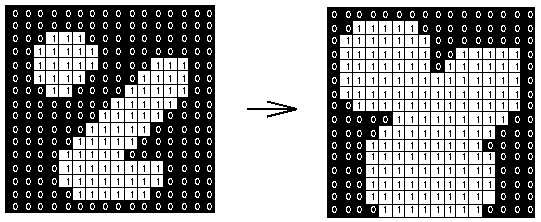
img_dilate = @. Gray(img > 0.9);
img_dilate1 = dilate(img_dilate)
img_dilate2 = dilate(dilate(img_dilate))
mosaicview(img_dilate, img_dilate1, img_dilate2; nrow = 1)
Opening
Opening morphology operation is equivalent to dilate(erode(img)). In opening(img, [region]), region allows you to control the dimensions over which this operation is performed. Opening can remove small bright spots (i.e. “salt”) and connect small dark cracks.
img_opening = @. Gray(1 * img > 0.5);
img_opening1 = opening(img_opening)
img_opening2 = opening(opening(img_opening))
mosaicview(img_opening, img_opening1, img_opening2; nrow = 1)
Closing
Closing morphology operation is equivalent to erode(dilate(img)). In closing(img, [region]), region allows you to control the dimensions over which this operation is performed. Closing can remove small dark spots (i.e. “pepper”) and connect small bright cracks.
img_closing = @. Gray(1 * img > 0.5);
img_closing1 = closing(img_closing)
img_closing2 = closing(closing(img_closing))
mosaicview(img_closing1, img_closing1, img_closing2; nrow = 1)
Tophat
Tophat is defined as the image minus its morphological opening. In tophat(img, [region]), region allows you to control the dimensions over which this operation is performed. This operation returns the bright spots of the image that are smaller than the structuring element.
img_tophat = @. Gray(1 * img > 0.2);
img_tophat1 = tophat(img_tophat)
img_tophat2 = tophat(tophat(img_tophat))
mosaicview(img_tophat, img_tophat1, img_tophat2; nrow = 1)
Bottom Hat
Bottom Hat morphology operation is defined as image's morphological closing minus the original image. In bothat(img, [region]), region allows you to control the dimensions over which this operation is performed. This operation returns the dark spots of the image that are smaller than the structuring element.
img_bothat = @. Gray(1 * img > 0.5);
img_bothat1 = bothat(img_tophat)
img_bothat2 = bothat(bothat(img_tophat))
img_bothat3 = bothat(bothat(bothat(img_tophat)))
mosaicview(img_bothat, img_bothat1, img_bothat2; nrow = 1)
Morphology Gradient
Morphological gradient returns morphological gradient of the image, which is the difference between the dilation and the erosion of a given image. In morphogradient(img, [region]), region allows you to control the dimensions over which this operation is performed.
img_gray = @. Gray(0.8 * img > 0.7);
img_morphograd = morphogradient(@. Gray(0.8 * img > 0.4))
mosaicview(img_gray, img_morphograd; nrow = 1)
Morphological Laplace
Morphological Laplace performs Morphological Laplacian of an image, which is defined as the arithmetic difference between the internal and the external gradient. In morpholaplace(img, [region]), region allows you to control the dimensions over which this operation is performed.
img_gray = @. Gray(0.8 * Gray.(img) > 0.7);
img_morpholap = morpholaplace(img_gray)
mosaicview(img_gray, img_morpholap; nrow = 1)
Reference
- Basic morphological operations in HIPR developed by Dr. R. Fisher et al : link
This page was generated using DemoCards.jl and Literate.jl.