ImageFiltering.jl

ImageFiltering supports linear and nonlinear filtering operations on arrays, with an emphasis on the kinds of operations used in image processing. The core function is imfilter, and common kernels (filters) are organized in the Kernel and KernelFactors modules.

Demonstration

Let's start with a simple example of linear filtering:

julia> using ImageFiltering, TestImages

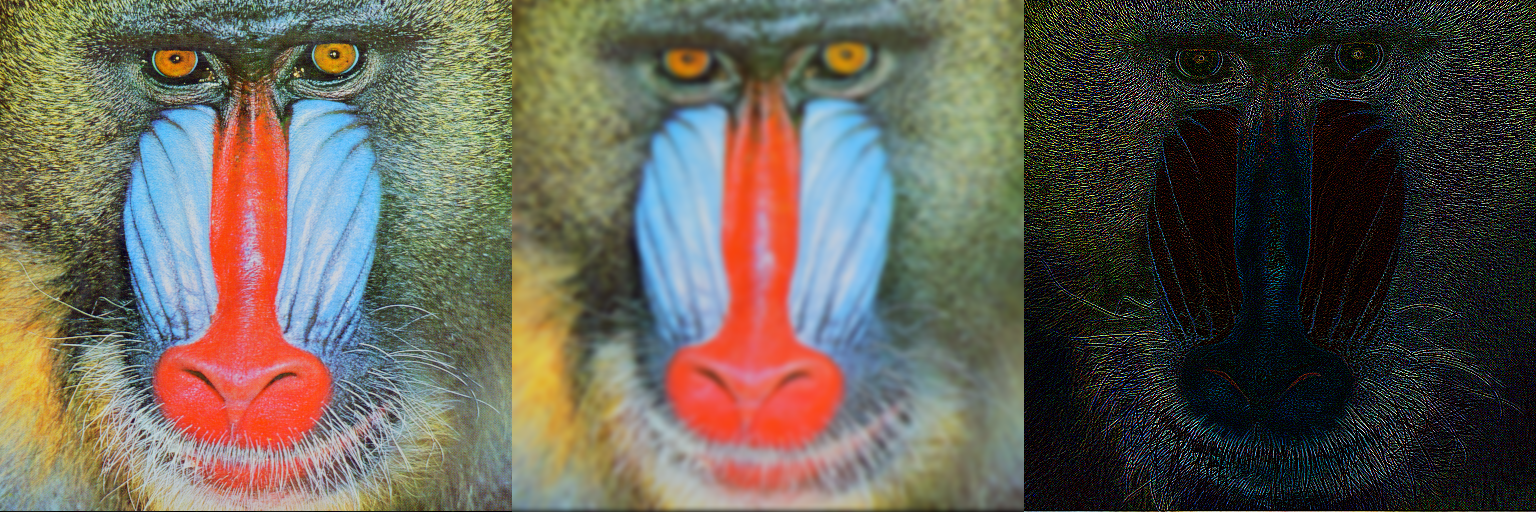
julia> img = testimage("mandrill");

julia> imgg = imfilter(img, Kernel.gaussian(3));

julia> imgl = imfilter(img, Kernel.Laplacian());

When displayed, these three images look like this:

The most commonly used function for filtering is imfilter.

Linear filtering: noteworthy features

Correlation, not convolution

ImageFiltering uses the following formula to calculate the filtered image F from an input image A and kernel K:

Consequently, the resulting image is the correlation, not convolution, of the input and the kernel. If you want the convolution, first call reflect on the kernel.

Kernel indices

ImageFiltering exploits a feature introduced into Julia 0.5, the ability to define arrays whose indices span an arbitrary range:

julia> Kernel.gaussian(1)
OffsetArrays.OffsetArray{Float64,2,Array{Float64,2}} with indices -2:2×-2:2:
 0.00296902  0.0133062  0.0219382  0.0133062  0.00296902
 0.0133062   0.0596343  0.0983203  0.0596343  0.0133062
 0.0219382   0.0983203  0.162103   0.0983203  0.0219382
 0.0133062   0.0596343  0.0983203  0.0596343  0.0133062
 0.00296902  0.0133062  0.0219382  0.0133062  0.00296902

The indices of this array span the range -2:2 along each axis, and the center of the gaussian is at position [0,0]. As a consequence, this filter "blurs" but does not "shift" the image; were the center instead at, say, [3,3], the filtered image would be shifted by 3 pixels downward and to the right compared to the original.

The centered function is a handy utility for converting an ordinary array to one that has coordinates [0,0,...] at its center position:

julia> centered([1 0 1; 0 1 0; 1 0 1])
OffsetArrays.OffsetArray{Int64,2,Array{Int64,2}} with indices -1:1×-1:1:
 1  0  1
 0  1  0
 1  0  1

See OffsetArrays for more information.

Factored kernels

A key feature of Gaussian kernels–-along with many other commonly-used kernels–-is that they are separable, meaning that K[j_1,j_2,...] can be written as $K_1[j_1] K_2[j_2] \cdots$. As a consequence, the correlation

can be written

If the kernel is of size m×n, then the upper version line requires mn operations for each point of filtered, whereas the lower version requires m+n operations. Especially when m and n are larger, this can result in a substantial savings.

To enable efficient computation for separable kernels, imfilter accepts a tuple of kernels, filtering the image by each sequentially. You can either supply m×1 and 1×n filters directly, or (somewhat more efficiently) call kernelfactors on a tuple-of-vectors:

julia> kern1 = centered([1/3, 1/3, 1/3])
OffsetArrays.OffsetArray{Float64,1,Array{Float64,1}} with indices -1:1:
 0.333333
 0.333333
 0.333333

julia> kernf = kernelfactors((kern1, kern1))
(ImageFiltering.KernelFactors.ReshapedOneD{Float64,2,0,OffsetArrays.OffsetArray{Float64,1,Array{Float64,1}}}([0.333333,0.333333,0.333333]),ImageFiltering.KernelFactors.ReshapedOneD{Float64,2,1,OffsetArrays.OffsetArray{Float64,1,Array{Float64,1}}}([0.333333,0.333333,0.333333]))

julia> kernp = broadcast(*, kernf...)
OffsetArrays.OffsetArray{Float64,2,Array{Float64,2}} with indices -1:1×-1:1:
 0.111111  0.111111  0.111111
 0.111111  0.111111  0.111111
 0.111111  0.111111  0.111111

julia> imfilter(img, kernf) ≈ imfilter(img, kernp)
true

If the kernel is a two dimensional array, imfilter will attempt to factor it; if successful, it will use the separable algorithm. You can prevent this automatic factorization by passing the kernel as a tuple, e.g., as (kernp,).

Popular kernels in Kernel and KernelFactors modules

The two modules Kernel and KernelFactors implement popular kernels in "dense" and "factored" forms, respectively. Type ?Kernel or ?KernelFactors at the REPL to see which kernels are supported.

A common task in image processing and computer vision is computing image gradients (derivatives), for which there is the dedicated function imgradients.

Automatic choice of FIR or FFT

For linear filtering with a finite-impulse response filtering, one can either choose a direct algorithm or one based on the fast Fourier transform (FFT). By default, this choice is made based on kernel size. You can manually specify the algorithm using Algorithm.FFT() or Algorithm.FIR().

Multithreading

If you launch Julia with JULIA_NUM_THREADS=n (where n > 1), then FIR filtering will by default use multiple threads. You can control the algorithm by specifying a resource as defined by ComputationalResources. For example, imfilter(CPU1(Algorithm.FIR()), img, ...) would force the computation to be single-threaded.

Arbitrary operations over sliding windows

This package also exports mapwindow, which allows you to pass an arbitrary function to operate on the values within a sliding window.

mapwindow has optimized implementations for some functions (currently, extrema).