ImageSegmentation.jl

Introduction

Image Segmentation is the process of partitioning the image into regions that have similar attributes. Image segmentation has various applications e.g, medical image segmentation, image compression and is used as a preprocessing step in higher level vision tasks like object detection and optical flow. This package is a collection of image segmentation algorithms written in Julia.

Installation

(v1.0) pkg> add ImageSegmentation

Example

Image segmentation is not a mathematically well-defined problem: for example, the only lossless representation of the input image would be to say that each pixel is its own segment. Yet this does not correspond to our own intuitive notion that some pixels are naturally grouped together. As a consequence, many algorithms require parameters, often some kind of threshold expressing your willingness to tolerate a certain amount of variation among the pixels within a single segment.

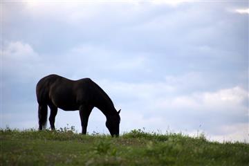
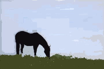
Let's see an example on how to use the segmentation algorithms in this package. We will try to separate the horse, the ground and the sky in the image below. We will explore two algorithms - seeded region growing and felzenszwalb. Seeded region growing requires us to know the number of segments and some points on each segment beforehand whereas felzenszwalb uses a more abstract parameter controlling degree of within-segment similarity.

Original

source

The documentation for seeded_region_growing says that it needs two arguments - the image to be segmented and a set of seed points for each region. The seed points have to be stored as a vector of (position, label) tuples, where position is a CartesianIndex and label is an integer. We will start by opening the image using ImageView and reading the coordinates of the seed points.

using Images, ImageView

img = load("src/pkgs/segmentation/assets/horse.jpg")
imshow(img)

Hover over the different objects you'd like to segment, and read out the coordinates of one or more points inside each object. We will store the seed points as a vector of (seed position, label) tuples and use seeded_region_growing with the recorded seed points.

using ImageSegmentation
seeds = [(CartesianIndex(126,81),1), (CartesianIndex(93,255),2), (CartesianIndex(213,97),3)]
segments = seeded_region_growing(img, seeds)

# output

Segmented Image with:
  labels map: 240×360 Matrix{Int64}
  number of labels: 3

All the segmentation algorithms (except Fuzzy C-means) return a struct SegmentedImage that stores the segmentation result. SegmentedImage contains a list of applied labels, an array containing the assigned label for each pixel, and mean color and number of pixels in each segment. This section explains how to access information about the segments.

julia> length(segment_labels(segments))
3

julia> segment_mean(segments)
Dict{Int64, RGB{Float64}} with 3 entries:
  2 => RGB{Float64}(0.793598,0.839543,0.932374)
  3 => RGB{Float64}(0.329863,0.35779,0.237457)
  1 => RGB{Float64}(0.0646509,0.0587034,0.0743471)

We can visualize each segment using its mean color:

julia> imshow(map(i->segment_mean(segments,i), labels_map(segments)));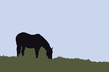

Original

This display form is used for many of the demonstrations below.

You can see that the algorithm did a fairly good job of segmenting the three objects. The only obvious error is the fact that elements of the sky that were "framed" by the horse ended up being grouped with the ground. This is because seeded_region_growing always returns connected regions, and there is no path connecting those portions of sky to the larger image. If we add some additional seed points in those regions, and give them the same label 2 that we used for the rest of the sky, we will get a result that is more or less perfect.

seeds = [(CartesianIndex(126,81), 1), (CartesianIndex(93,255), 2), (CartesianIndex(171,103), 2),
         (CartesianIndex(172,142), 2), (CartesianIndex(182,72), 2), (CartesianIndex(213,97), 3)]
segments = seeded_region_growing(img, seeds)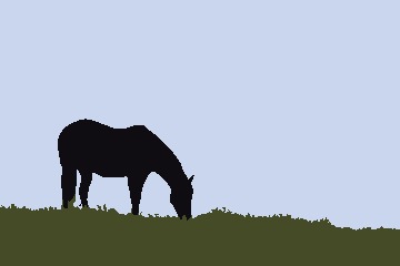

Original

Now let's segment this image using felzenszwalb algorithm. felzenszwalb only needs a single parameter k which controls the size of segments. Larger k will result in bigger segments. Using k=5 to k=500 generally gives good results.

julia> using Images, ImageSegmentation

julia> img = load("src/pkgs/segmentation/assets/horse.jpg");

julia> segments = felzenszwalb(img, 100)
Segmented Image with:
  labels map: 240×360 Matrix{Int64}
  number of labels: 43

julia> segments = felzenszwalb(img, 10)  #smaller segments but noisy segmentation
Segmented Image with:
  labels map: 240×360 Matrix{Int64}
  number of labels: 312

k = 100	k = 10

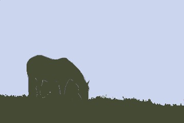We only got two "major" segments with k = 100. Setting k = 10 resulted in smaller but rather noisy segments. felzenzwalb also takes an optional argument min_size - it removes all segments smaller than min_size pixels. (Most methods don't remove small segments in their core algorithm. We can use the prune_segments method to postprocess the segmentation result and remove small segments.)

segments = felzenszwalb(img, 10, 100)  # removes segments with fewer than 100 pixels
imshow(map(i->segment_mean(segments,i), labels_map(segments)))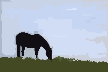

Original

Result

All segmentation algorithms (except Fuzzy C-Means) return a struct SegmentedImage as its output. SegmentedImage contains all the necessary information about the segments. The following functions can be used to get the information about the segments:

labels_map : It returns an array containing the labels assigned to each pixel
segment_labels : It returns a list of all the assigned labels
segment_mean : It returns the mean intensity of the supplied label.
segment_pixel_count : It returns the count of the pixels that are assigned the supplied label.

Demo

julia> img = fill(1, 4, 4);

julia> img[1:2,1:2] .= 2;

julia> img
4×4 Matrix{Int64}:
 2  2  1  1
 2  2  1  1
 1  1  1  1
 1  1  1  1

julia> seg = fast_scanning(img, 0.5);

julia> labels_map(seg) # returns the assigned labels map
4×4 Matrix{Int64}:
 1  1  3  3
 1  1  3  3
 3  3  3  3
 3  3  3  3

julia> segment_labels(seg) # returns a list of all assigned labels
2-element Vector{Int64}:
 1
 3

julia> segment_mean(seg, 1) # returns the mean intensity of label 1
2.0

julia> segment_pixel_count(seg, 1) # returns the pixel count of label 1
4

Algorithms

Seeded Region Growing

Seeded region growing segments an image with respect to some user-defined seeds. Each seed is a (position, label) tuple, where position is a CartesianIndex and label is a positive integer. Each label corresponds to a unique partition of the image. The algorithm tries to assign these labels to each of the remaining points. If more than one point has the same label then they will be contribute to the same segment.

Demo

julia> using Images, ImageSegmentation

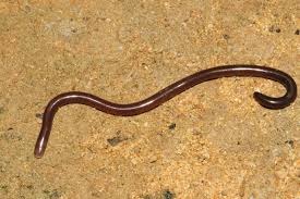
julia> img = load("src/pkgs/segmentation/assets/worm.jpg");

julia> seeds = [(CartesianIndex(104, 48), 1), (CartesianIndex( 49, 40), 1),
                (CartesianIndex( 72,131), 1), (CartesianIndex(109,217), 1),
                (CartesianIndex( 28, 87), 2), (CartesianIndex( 64,201), 2),
                (CartesianIndex(104, 72), 2), (CartesianIndex( 86,138), 2)];

julia> seg = seeded_region_growing(img, seeds)
Segmented Image with:
  labels map: 183×275 Matrix{Int64}
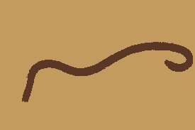
  number of labels: 2

Original (source):

Original

Segmented Image with labels replaced by their intensity means:

SegmentedImage

Unseeded Region Growing

This algorithm is similar to Seeded Region Growing but does not require any prior information about the seed points. The segmentation process initializes with region $A_1$ containing a single pixel of the image. Let an intermediate state of the algorithm consist of a set of identified regions $A_1, A_2, ..., A_n$. Let $T$ be the set of all unallocated pixels which borders at least one of these regions. The growing process involves selecting a point $z \in T$ and region $A_j$ where $j \in [ 1,n ]$ such that

\[\delta(z, A_j)= \min_{x \in T, k \in [ 1,n ] } \{ \delta(x, A_k)\}\]

where $\delta(x, A_i)= | \operatorname{img}(x) - \operatorname{mean}_{y \in A_i} [ \operatorname{img}(y) ] |$

If $\delta(z, A_j)$ is less than threshold then the pixel z is added to $A_j$. Otherwise we choose the most similar region $\alpha$ such that

\[\alpha = \argmin_{A_k} \{ \delta(z, A_k) \}\]

If $\delta(z, \alpha)$ is less than threshold then the pixel z is added to $\alpha$. If neither of the two conditions is satisfied, then the pixel is assigned a new region $A_{n+1}$. After assignment of $z$, we update the statistic of the assigned region. The algorithm halts when all the pixels have been assigned to some region.

unseeded_region_growing requires the image img and threshold as its parameters.

Demo

julia> using ImageSegmentation, Images

julia> img = load("src/pkgs/segmentation/assets/tree.jpg");

julia> seg = unseeded_region_growing(img, 0.05) # here 0.05 is the threshold
Segmented Image with:
  labels map: 320×480 Matrix{Int64}
  number of labels: 698

Threshold	Output	Compression percentage
Original (source)		0 %
0.05		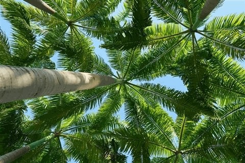60.63%
0.1		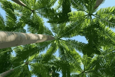71.27%
0.2		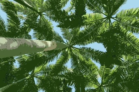79.96%

Felzenszwalb's Region Merging Algorithm

This algorithm operates on a Region Adjacency Graph (RAG). Each pixel/region is a node in the graph and adjacent pixels/regions have edges between them with weight measuring the dissimilarity between pixels/regions. The algorithm repeatedly merges similar regions till we get the final segmentation. It efficiently computes oversegmented “superpixels” in an image. The function can be directly called with an image (the implementation internally creates a RAG of the image first and then proceeds).

Demo

julia> using Images, ImageSegmentation, TestImages

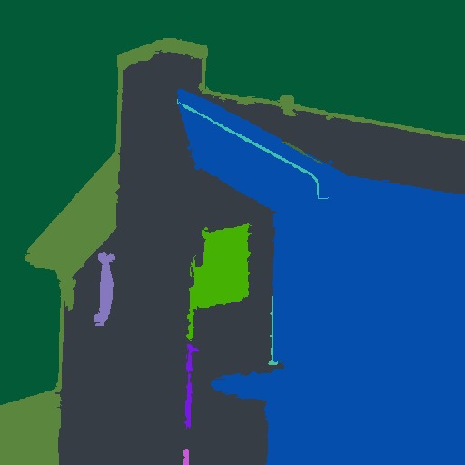
julia> img = Gray.(testimage("house"));

julia> segments = felzenszwalb(img, 300, 100) # k=300 (the merging threshold), min_size = 100 (smallest number of pixels/region)
Segmented Image with:
  labels map: 512×512 Matrix{Int64}
  number of labels: 11

Here let's visualize segmentation by creating an image with each label replaced by a random color:

function get_random_color(seed)
    Random.seed!(seed)
    rand(RGB{N0f8})
end
imshow(map(i->get_random_color(i), labels_map(segments)))

MeanShift Segmentation

MeanShift is a clustering technique. Its primary advantages are that it doesn't assume a prior on the shape of the cluster (e.g, gaussian for k-means) and we don't need to know the number of clusters beforehand. The algorithm doesn't scale well with size of image.

Demo

julia> using Images, ImageSegmentation, TestImages

julia> img = Gray.(testimage("house"));

julia> img = imresize(img, (128, 128));

julia> segments = meanshift(img, 16, 8/255) # parameters are smoothing radii: spatial=16, intensity-wise=8/255
Segmented Image with:
  labels map: 128×128 Matrix{Int64}
  number of labels: 44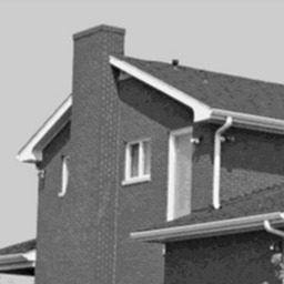

Fast Scanning

Fast scanning algorithm segments the image by scanning it once and comparing each pixel to its upper and left neighbor. The algorithm starts from the first pixel and assigns it to a new segment $A_1$. Label count lc is assigned 1. Then it starts a column-wise traversal of the image and for every pixel, it computes the difference measure diff_fn between the pixel and its left neighbor, say $\delta_{l}$ and between the pixel and its top neighbor, say $\delta_{t}$. Four cases arise:

$\delta_{l} \ge$ threshold and $\delta_{t} <$ threshold : We can say that the point has similar intensity to that its top neighbor. Hence, we assign the point to the segment that contains its top neighbor.
$\delta_{l} <$ threshold and $\delta_{t} \ge$ threshold : Similar to case 1, we assign the point to the segment that contains its left neighbor.
$\delta_{l} \ge$ threshold and $\delta_{t} \ge$ threshold : Point is significantly different from its top and left neighbors and is assigned a new label $A_{\text{lc}+1}$ and lc is incremented.
$\delta_{l} <$ threshold and $\delta_{t} <$ threshold : In this case, we merge the top and left segments together and assign the point under consideration to this merged segment.

This algorithm segments the image in just two passes (one for segmenting and other for merging), hence it is very fast and can be used in real time applications.

Time Complexity: $O(n)$ where $n$ is the number of pixels

Demo

julia> using ImageSegmentation, TestImages

julia> img = testimage("camera");

julia> seg = fast_scanning(img, 0.1)  # threshold = 0.1
Segmented Image with:
  labels map: 512×512 Matrix{Int64}
  number of labels: 2538

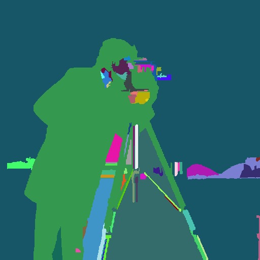
julia> seg = prune_segments(seg, i->(segment_pixel_count(seg,i)<50), (i,j)->(-segment_pixel_count(seg,j)))
Segmented Image with:
  labels map: 512×512 Matrix{Int64}
  number of labels: 65

Original:

Original

Segmented Image:

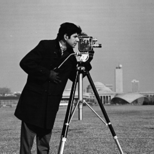
SegmentedImage

Region Splitting using RegionTrees

This algorithm follows the divide and conquer methodology. If the input image is homogeneous then nothing is to be done. In the other case, the image is split into two across every dimension and the smaller parts are segmented recursively. This procedure generates a region tree which can be used to create a segmented image.

Time Complexity: $O(n \log(n))$ where $n$ is the number of pixels

Demo

julia> using TestImages, ImageSegmentation

julia> img = testimage("lena_gray");

julia> function homogeneous(img)
           min, max = extrema(img)
           max - min < 0.2
       end
homogeneous (generic function with 1 method)

julia> seg = region_splitting(img, homogeneous)
Segmented Image with:
  labels map: 256×256 Matrix{Int64}
  number of labels: 8836

Original:

Original

Segmented Image with labels replaced by their intensity means:

SegmentedImage

Fuzzy C-means

Fuzzy C-means clustering is widely used for unsupervised image segmentation. It is an iterative algorithm which tries to minimize the cost function:

\[J = \displaystyle\sum_{i=1}^{N} \sum_{j=1}^{C} \delta_{ij} \| x_{i} - c_{j} \|^2\]

Unlike K-means, it allows pixels to belong to two or more clusters. It is widely used for medical imaging like in the soft segmentation of brain tissue model. Note that both Fuzzy C-means and K-means have an element of randomness, and it's possible to get results that vary considerably from one run to the next.

Time Complexity: $O(n \cdot C^2 \cdot \text{iter})$ where $n$ is the number of pixels, $C$ is number of clusters and $\text{iter}$ is the number of iterations.

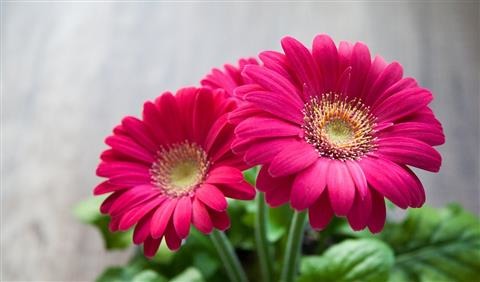
Demo

julia> using ImageSegmentation, Images

julia> img = load("src/pkgs/segmentation/assets/flower.jpg");

julia> r = fuzzy_cmeans(img, 3, 2)
FuzzyCMeansResult: 3 clusters for 135360 points in 3 dimensions (converged in 27 iterations)

Briefly, r contains two fields of interest:

centers, a 3×C matrix of center positions for C clusters in RGB colorspace. You can extract it as a vector of colors using centers = colorview(RGB, r.centers).
weights, a n×C matrix such that r.weights[10,2] would be the weight of the 10th pixel in the green color channel (color channel 2). You can visualize this component as centers[i]*reshape(r.weights[:,i], axes(img)).

See the documentation in Clustering.jl for further details.

Original (source)

Original

Output with pixel intensity = cluster center intensity * membership of pixel in that class

Magenta petals	Greenish Leaves	White background

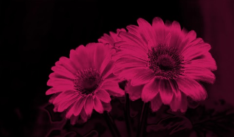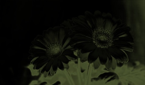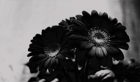Watershed

The watershed algorithm treats an image as a topographic surface where bright pixels correspond to peaks and dark pixels correspond to valleys. The algorithm starts flooding from valleys (local minima) of this topographic surface and region boundaries are formed when water from different sources merge. If the image is noisy, this approach leads to oversegmetation. To prevent oversegmentation, marker-based watershed is used i.e. the topographic surface is flooded from a predefined set of markers.

Let's see an example on how to use watershed to segment touching objects. To use watershed, we need to modify the image such that in the new image flooding the topographic surface from the markers separates each coin. If this modified image is noisy, flooding from local minima may lead to oversegmentation and so we also need a way to find the marker positions. In this example, the inverted distance_transform of the thresholded image (dist image) has the required topographic structure (This page explains why this works). We can threshold the dist image to get the marker positions.

Demo

julia> using Images, ImageSegmentation

julia> img = load(download("http://docs.opencv.org/3.1.0/water_coins.jpg"));

julia> bw = Gray.(img) .> 0.5;

julia> dist = 1 .- distance_transform(feature_transform(bw));

julia> markers = label_components(dist .< -15);

julia> segments = watershed(dist, markers)
Segmented Image with:
  labels map: 312×252 Matrix{Int64}
  number of labels: 24

julia> imshow(map(i->get_random_color(i), labels_map(segments)) .* (1 .-bw))       #shows segmented image

Original Image	Thresholded Image

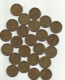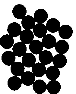Inverted Distance Transform Image	Markers

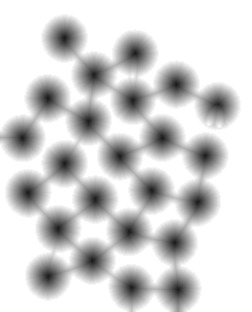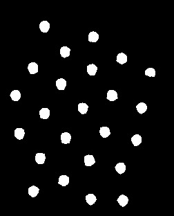Segmented Image

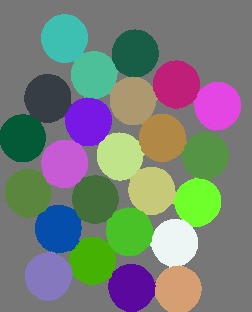Some helpful functions

Creating a Region Adjacency Graph (RAG)

A region adjacency graph can directly be constructed from a SegmentedImage using the region_adjacency_graph function. Each segment is denoted by a vertex and edges are constructed between adjacent segments. The output is a tuple of SimpleWeightedGraph and a Dict(label=>vertex) with weights assigned according to weight_fn.

julia> using ImageSegmentation, Distances, TestImages

julia> img = testimage("camera");

julia> seg = felzenszwalb(img, 10, 100);

julia> weight_fn(i,j) = euclidean(segment_pixel_count(seg,i), segment_pixel_count(seg,j));

julia> G, vert_map = region_adjacency_graph(seg, weight_fn);

julia> G
{70, 139} undirected simple Int64 graph with Float64 weights

Here, the difference in pixel count has been used as the weight of the connecting edges. This difference measure can be useful if one wants to use this region adjacency graph to remove smaller segments by merging them with their neighbouring largest segment. Another useful difference measure is the euclidean distance between the mean intensities of the two segments.

Creating a Region Tree

A region tree can be constructed from an image using region_tree function. If the image is not homogeneous, then it is split into half along each dimension and the function is called recursively for each portion of the image. The output is a RegionTree.

julia> using ImageSegmentation

julia> function homogeneous(img)
           min, max = extrema(img)
           max - min < 0.2
       end
homogeneous (generic function with 1 method)

julia> t = region_tree(img, homogeneous)        # `img` is an image
Cell: RegionTrees.HyperRectangle{2, Float64}([1.0, 1.0], [300.0, 300.0])

For more information regarding RegionTrees, see this.

Pruning unnecessary segments

All the unnecessary segments can be easily removed from a SegmentedImage using prune_segments. It removes a segment by replacing it with the neighbor which has the least value of diff_fn. A list of the segments to be removed can be supplied. Alternately, a function can be supplied that returns true for the labels that must be removed.

Note

The resultant SegmentedImage might have the different labels compared to the original SegmentedImage.

For this example and the next one (in Removing a segment), a sample SegmentedImage has been used. It can be generated as:

julia> img = fill(1, (4, 4));

julia> img[3:4,:] .= 2;

julia> img[1:2,3:4] .= 3;

julia> seg = fast_scanning(img, 0.5);

julia> labels_map(seg)
4×4 Matrix{Int64}:
 1  1  3  3
 1  1  3  3
 2  2  2  2
 2  2  2  2

julia> seg.image_indexmap
4×4 Matrix{Int64}:
 1  1  3  3
 1  1  3  3
 2  2  2  2
 2  2  2  2

julia> diff_fn(rem_label, neigh_label) = segment_pixel_count(seg,rem_label) - segment_pixel_count(seg,neigh_label);

julia> new_seg = prune_segments(seg, [3], diff_fn);

julia> labels_map(new_seg)
4×4 Matrix{Int64}:
 1  1  2  2
 1  1  2  2
 2  2  2  2
 2  2  2  2

Removing a segment

If only one segment is to be removed, then rem_segment! can be used. It removes a segment from a SegmentedImage in place, replacing it with the neighbouring segment having least diff_fn value.

Note

If multiple segments need to be removed then prune_segments should be preferred as it is much more time efficient than calling rem_segment! multiple times.

julia> seg.image_indexmap
4×4 Matrix{Int64}:
 1  1  3  3
 1  1  3  3
 2  2  2  2
 2  2  2  2

julia> diff_fn(rem_label, neigh_label) = segment_pixel_count(seg,rem_label) - segment_pixel_count(seg,neigh_label);

julia> rem_segment!(seg, 3, diff_fn);

julia> labels_map(new_seg)
4×4 Matrix{Int64}:
 1  1  2  2
 1  1  2  2
 2  2  2  2
 2  2  2  2