Arrays, Numbers, and Colors
In Julia, an image is just an array, and many of the ways you manipulate images come from the general methods to work with multidimensional arrays. For example,
julia> img = rand(2,2)
2×2 Matrix{Float64}:
 0.366796  0.210256
 0.523879  0.819338
defines an "image" img of 64-bit floating-point numbers. You should be able to use this as an image in most or all functions in JuliaImages.
We'll be talking quite a bit about handling arrays. This page will focus on the "element type" (eltype) stored in the array. In case you're new to Julia, if a is an array of integers:
julia> a = [1,2,3,4]
4-element Vector{Int64}:
 1
 2
 3
 4
then either of the following creates a new array where the element type is Float64:
map(Float64, a)
Float64.(a)     # short for broadcast(Float64, a)
For example,
julia> Float64.(a)
4-element Vector{Float64}:
 1.0
 2.0
 3.0
 4.0
Arrays are indexed with square brackets (a[1]), with indexing starting at 1 by default. A two-dimensional array like img can be indexed as img[2,1], which would be the second row, first column. Julia also supports "linear indexing," using a single integer to address elements of an arbitrary multidimensional array in a manner that (in simple cases) reflects the memory offset of the particular element. For example, img[3] corresponds to img[1,2] (numbering goes down columns, and then wraps around at the top of the next column, because Julia arrays are stored in "column major" order where the fastest dimension is the first dimension).
Numbers versus colors
For the array img we created above, you can display it as a grayscale image using ImageView. But if you happen to be following along in Juno or IJulia, you might notice that img does not display as an image: instead, it prints as an array of numbers as shown above. Arrays of "plain numbers" are not displayed graphically, because they might represent something numerical (e.g., a matrix used for linear algebra) rather than an image. To indicate that this is worthy of graphical display, convert the element type to a color chosen from the Colors package:
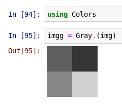
Here we used Gray to indicate that this array should be interpreted as a grayscale image. (Note that the Images package re-exports Colors, so you can alternatively say using Images.)
Under the hood, what is Gray doing? It's informative to see the "raw" object, displayed as text:
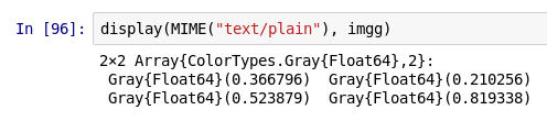
(Users of Juno or the Julia command-line REPL interface will see this representation immediately.)
You can see this is a 2×2 array of Gray{Float64} objects. You might be curious how these Gray objects are represented. In the command-line REPL, it looks like this (the same command works with IJulia):
julia> dump(imgg[1,1])
ColorTypes.Gray{Float64}
  val: Float64 0.36679641243992434
dump shows the "internal" representation of an object. You can see that Gray is a type (technically, an immutable struct) with a single field val; for Gray{Float64}, val is a 64-bit floating point number. Using val directly is not recommended: you can extract the Float64 value with the accessor functions real or gray (the reason for the latter name will be clearer when we discuss RGB colors).
What kind of overhead do these objects incur?
julia> sizeof(img)
32

julia> sizeof(imgg)
32
The answer is "none": they don't take up any memory of their own, nor do they typically require any additional processing time. The Gray "wrapper" is just an interpretation of the values, one that helps clarify that this should be displayed as a grayscale image. Indeed, img and imgg compare as equal:
julia> img == imgg
true
There's more to say on this topic, but we'll wait until we discuss Conversions vs. views.
Colors beyond the pale
Gray is not the only color in the universe:
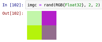
Let's look at imgc as text (shown here in the REPL):
julia> imgc
2×2 Array{ColorTypes.RGB{Float32},2}:
 RGB{Float32}(0.75509,0.965058,0.65486)     RGB{Float32}(0.696203,0.142474,0.783316)
 RGB{Float32}(0.705195,0.953892,0.0744661)  RGB{Float32}(0.571945,0.42736,0.548254)

julia> size(imgc)
(2,2)

julia> dump(imgc[1,1])
ColorTypes.RGB{Float32}
  r: Float32 0.7550899
  g: Float32 0.9650581
  b: Float32 0.65485954
Here we see one of the primary differences between Julia's approach to images and that of several other popular frameworks: imgc does not have a dimension of the array devoted to the "color channel." Instead, every element of the array corresponds to a complete pixel's worth of information. Often this simplifies the logic of many algorithms, sometimes allowing a single implementation to work for both color and grayscale images.
You can extract the individual color channels using their field names (r, g, and b), but as you'll see in a moment, a more universal approach is to use accessor functions:
julia> c = imgc[1,1]; (red(c), green(c), blue(c))
(0.7550899f0,0.9650581f0,0.65485954f0)
Julia's Colors package allows the same color to be represented in several different ways, and this can facilitate interaction with other tools. For example, certain C libraries permit or prefer the order of the color channels to be different:
julia> dump(BGR(c))
ColorTypes.BGR{Float32}
  b: Float32 0.65485954
  g: Float32 0.9650581
  r: Float32 0.7550899
or even to pack the red, green, and blue colors—together with a dummy "alpha" (transparency) channel—into a single 32-bit integer:
julia> c24 = RGB24(c); dump(c24)
ColorTypes.RGB24
  color: UInt32 12711591

julia> c24.color
0x00c1f6a7
From first (the first two hex-digits after the "0x") to last (the final two hex-digits), the order of the channels here is alpha, red, green, blue:
julia> 0xc1/0xff
0.7568627450980392

julia> 0xf6/0xff
0.9647058823529412

julia> 0xa7/0xff
0.6549019607843137
These values are close to the channels of c, but have been rounded off—each channel is encoded with only 8 bits, so some approximation of the exact floating-point value is unavoidable.
A consistent scale for floating-point and "integer" colors: fixed-point numbers
c24 does not have an r field, but we can still use red to extract the red channel:
julia> r = red(c24)
0.757N0f8
This may look fairly strange at first, so let's unpack this carefully. Notice first that the "floating-point" portion of this number matches (to within the precision of the rounding) the value of red(c). The N0f8 means "Normalized with 8 fractional bits, with 0 bits left for representing values higher than 1." This is a fixed-point number—rather like floating-point numbers, except that the decimal does not "float". Internally, these are represented in terms of the 8-bit unsigned integer UInt8
julia> dump(r)
FixedPointNumbers.N0f8
  i: UInt8 193
(Note that N0f8 is an abbreviation; the full typename is Normed{UInt8, 8}.) N0f8 interprets this 8-bit integer as a value lying between 0 and 1, with 0 corresponding to 0x00 and 1 corresponding to 0xff. This interpretation affects how the number is used for arithmetic and conversion to and from other values. Stated another way, r behaves as
julia> r == 193/255
true
for essentially all purposes (but see A note on arithmetic overflow).
This has a very important consequence: in many other image frameworks, the "meaning" of an image depends on how it is stored, but in Julia the meaning can be assigned independently of storage representation. For example, in a different language/framework, the following sequence:
img = uint8(255*rand(10, 10, 3));
figure; image(img)
imgd = double(img);   % convert to double-precision, but don't change the values
figure; image(imgd)
might produce the following images:
| img | imgd |
|---|---|
 |  |
The one on the right looks white because floating-point types are interpreted on a 0-to-1 colorscale (and all of the entries in img happen to be 1 or higher), whereas uint8 is interpreted on a 0-to-255 colorscale. Unfortunately, two arrays that are numerically identical have very different meanings as images.
Many frameworks offer convenience functions for converting images from one representation to another, but this can be a source of bugs if we go to compare images: in most number systems we would agree that 255 != 1.0, and this fact means that you sometimes need to be quite careful when converting from one representation to another. Conversely, using these Julia packages there is no discrepancy in "meaning" between the encoding of images represented as floating point or 8-bit (or 16-bit) fixed-point numbers: 0 always means "black" and 1 or something greater than 1 always means "white" or "saturated."
Now, this doesn't prevent you from constructing pixels with values out of this range:
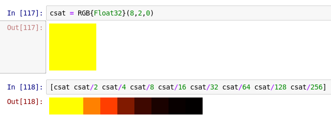
Notice that the first two yellows look identical, because both the red and green color channels are 1 or higher and consequently are saturated.
However, you should be aware that for integer inputs, the default is to use the N0f8 element type, and this type cannot represent values outside the range from 0 to 1:
julia> RGB(8,2,0)ERROR: ArgumentError: (8, 2, 0) are integers in the range 0-255, but integer inputs are encoded with the N0f8
  type, an 8-bit type representing 256 discrete values between 0 and 1.
  Consider dividing your input values by 255, for example: RGB{N0f8}(8/255,2/255,0/255)
  Or use `reinterpret(N0f8, x)` if `x` is a `UInt8`.
  See the READMEs for FixedPointNumbers and ColorTypes for more information.
The error message here reminds you how to resolve a common mistake, trying to construct red as RGB(255, 0, 0). In Julia, that should always be RGB(1, 0, 0).
More fixed-point numbers
16-bit images can be expressed in terms of the N0f16 type. Let's compare the maximum values (typemax) and smallest-difference (eps) representable with N0f8 and N0f16:
julia> using FixedPointNumbers

julia> (typemax(N0f8), eps(N0f8))
(1.0N0f8, 0.004N0f8)

julia> (typemax(N0f16), eps(N0f16))
(1.0N0f16, 2.0e-5N0f16)
You can see that this type also has a maximum value of 1, but is higher precision, with the gap between adjacent numbers being much smaller.
Many cameras (particularly, scientific cameras) now return 16-bit values. However, some cameras do not provide a full 16 bits worth of information; for example, the camera might be 12-bit and return values between 0x0000 and 0x0fff. As an N0f16, the latter displays as nearly black:

Since the camera is saturated, this is quite misleading—it should instead display as white.
This again illustrates one of the fundamental problems about assuming that the representation (a 16-bit integer) also describes the meaning of the number. In Julia, we decouple these by providing many different fixed-point number types. In this case, the natural way to interpret these values is by using a fixed-point number with 12 fractional bits; this leaves 4 bits that we can use to represent values bigger than 1, so the number type is called N4f12:
julia> (typemax(N4f12), eps(N4f12))
(16.0037N4f12, 0.0002N4f12)
You can see that the maximum value achievable by an N4f12 is approximately 16 = 2^4.
Using this N4f12 interpretation of the 16 bits, the color displays correctly as white:

and acts like 1 for all arithmetic purposes. Even though the raw representation as 0x0fff is the same, we can endow the number with appropriate meaning through its type.
A note on arithmetic overflow
Sometimes, being able to construct a color values outside 0 to 1 is useful. For example, if you want to compute the average color in an image, the natural approach is to first sum all the pixels and then divide by the total number of pixels. At an intermediate stage, the sum will typically result in a color that is well beyond saturation.
It's important to note that arithmetic with N0f8 numbers, like arithmetic with UInt8, overflows:
julia> 0xff + 0xff
0xfe

julia> 1N0f8 + 1N0f8
0.996N0f8

julia> 0xfe/0xff      # the first result corresponds to the second result
0.996078431372549
Consequently, if you're accumulating values, it's advisable to accumulate them in an appropriate floating-point type, such as Float32, Gray{Float64}, or RGB{Float32}.